
Furiosa Chip

Furiosa 사의 NPU는 총 2가지가 있는데 1세대 Warboy는 computer vision에 특화되어 있으며, 2세대 RNGD는 LLM과 Multimodality(다중 모드 작업 지원)에 특화되어 있으며 전 세계 최초로 HBM을 사용했다는 특징이 있습니다.
Process of using AI Service using WARBOY
*본문에서는 다음 그림의 진행과정에 따라 내용을 전개하므로 다음 과정을 잘 알아두면 좋겠다.
- DL Framework : AI 모델을 개발하는 딥러닝 프레임워크
- Export ONNX : 현재 Warboy SDK 에서는 TFLite, ONNX 모델을 지원하고 있기 때문에, PyTorch와 같은 DL Framework에서 개발한 모델을 TFLite 혹은 ONNX로 변환하는 과정이 필요함
- ONNX(Open Neural Network Exchange) Graph : ONNX 형식의 모델 그래프입니다.
- Furiosa Quantizer : Inference 최적화를 위해 WARBOY는 8-bit 정수형 모델을 기반으로 동작하며, WARBOY에서 모델을 실행하기 위해 8-bit 정수형 모델로의 변환이 필요하며 이 과정을 Quantization이라 함
- ONNX Graph(8 bit integer) : 양자화된 8 bit integer 형식의 ONNX 그래프
- Furiosa Compiler : Furiosa SDK는 compiler를 제공하고 이를 통해 WARBOY에 최적화된 프로그램을 생성하고, 또한 이를 실행할 수 있는 다양한 Runtime을 제공함으로써 사용자들이 WARBOY 기반의 AI서비스를 효과적으로 실행할 수 있음
- Warboy ISA : AI 모델이 실행되는 최종 단계
- Debugger, profiler : Useful tool for optimization
- Furiosa SDK는 사용자들이 NPU를 활용해 DL 서비스의 성능을 최적화할 수 있도록 프로파일링 및 디버깅 도구 제공하고 있음
8 bit integer 형식이 inference 최적화에 적합한 이유 :
1. 메모리 효율성 : 8-bit 정수는 32-bit 부동소수점에 비해 메모리 사용량을 크게 줄일 수 있습니다. 이는 모델 크기를 줄이고 메모리 대역폭 요구사항을 감소시킵니다.
2. 연산 속도 : 많은 하드웨어에서 정수 연산이 부동소수점 연산보다 빠릅니다.
3. 에너지 효율성: 정수 연산은 일반적으로 부동소수점 연산보다 에너지 효율적입니다. 이는 배터리 수명이 중요한 모바일 기기에서 특히 중요

Installing Furiosa SDK

1. API server registration
FuriosaAI가 제공하는 SW 요소들을 사용하기 위해서, NPU 장치의 Driver, Firmware 그리고 Runtime 패키지들을 APT 서버를 통해 설치할 수 있으며, 이를 위해 APT 서버를 설정하는 과정이 필요함.
- 1. HTTPS 기반의 APT 서버 접근을 위해 필요 패키지 설치
sudo apt update
sudo apt install -y ca-certificates apt-transport-https gnupg wget
- 2. Furiosa AI의 공개 signing key 등록
mkdir -p /etc/apt/keyrings && \
wget -q -O- https://archive.furiosa.ai/furiosa-apt-key.gpg \
| gpg --dearmor \
| sudo tee /etc/apt/keyrings/furiosa-apt-key.gpg > /dev/null
- 3. Furiosa AI 개발자 센터에서 API 키를 발급하고 발급한 API 키를 아래와 같이 설정
아래 코드의 Key(ID)와 Password는 따로 발급받아야 합니다.
sudo tee -a /etc/apt/auth.conf.d/furiosa.conf > /dev/null <<EOT
  machine archive.furiosa.ai
	login d844d9b3-98ec-460d-93a4-ecca65b2523c
	password w6GfiiQGMTJPMZz6SUAC7Q5g6IXM2ezGIBqtyPd3KqNdXxFeEfGlbtoKanQlQiLt
EOT

sudo chmod 400 /etc/apt/auth.conf.d/furiosa.conf
- 4. 리눅스 버전에 따라 APT 서버 설정 (Ubuntu 20.04, 22.04, 24.04 호환 가능)
sudo tee -a /etc/apt/sources.list.d/furiosa.list <<EOT
deb [arch=amd64 signed-by=/etc/apt/keyrings/furiosa-apt-key.gpg] https://archive.furiosa.ai/ubuntu focal restricted
EOT
2. APT 서버를 이용한 필수 패키지 설치
sudo apt-get update && sudo apt-get install -y furiosa-driver-warboy furiosa-libnux
3. 내 환경에 NPU가 있는지 확인
sudo apt-get install -y furiosa-toolkit
furiosactl info
현재 내 서버와 연결되어 있는 warboy npu하나가 존재한다는 것을 알 수 있습니다.
4. Conda 기반의 Python 개발 환경설정 및 Furiosa Python SDK 설치
wget https://repo.anaconda.com/miniconda/Miniconda3-latest-Linux-x86_64.sh
sh ./Miniconda3-latest-Linux-x86_64.sh
source ~/.bashrc
conda create -n furiosa-3.9 python=3.9
conda activate furiosa-3.9
파이썬 3.9.20 버전이 적용됨을 알 수 있습니다.
5. Furiosa Python SDK 설치
pip install furiosa-sdk[full]

6. Tutorial File
- 1. Installation
pip install gdown
sudo apt install unzip
gdown --id 17Ok3bAit8uFH1QO-TtZAlZpKvzS4ANCk
unzip warboy_tutorial.zip
- 2. Setup
cd warboy_tutorial
chmod 500 setup.sh
./setup.sh
1. Export ONNX

ONNX Graph
- ONNX (Open Neural Network Exchange)
- 다양한 DL Framework 간 상호운용성을 제공하기 위해 개발된 표준 모델 형식
- 이를 통해 딥러닝 모델을 서로 다른 Framework로전환하고 배포할 수 있음
- 생성된 ONNX 모델은 Netron tool을 통해 시각화할 수 있으며, ONNX 모델과 이를 이루고 있는 Tensor들의 정보를 확인 가능
- Netron
Netron
netron.app
#export_onnx.py
import torch
from ultralytics import YOLO

# 1. load to pytorch model
torch_model = YOLO("yolov8n.pt").model
torch_model.eval()

# 2. define sample input
sample_input = torch.zeros(1, 3, 640, 640) batch size : 1, channel : 3, image size : 640*640

# 3. convert PyTorch to ONNX
torch.onnx.export(
    torch_model,
    sample_input,
    "yolov8n.onnx",
    opset_version = 13,
    input_names = ["images"],
    output_names = ["outputs"]
)
하지만 위 그림에서는 문제점이 있습니다.

각 anchor에서 클래스의 결과와 box 결과를 채널 축으로 하는 concat 연산자에서 양자화 이후 정확도가 떨어지는 문제가 발생하기 때문에 위의 그림(모델 결과를 decode)하는 부분을 제거하여 edit_onnx.py를 통해 yolov8n.onnx를 수정하였습니다.
#edit_onnx.py
import onnx
from onnx.utils import Extractor

def edit_onnx_graph(model, input_name, input_shape):
    output_to_shape = []

    for idx in range(3):
        box_layer = (
            f"/model.22/cv2.{idx}/cv2.{idx}.2/Conv_output_0",
            (1, 64, int(input_shape[2] / (8 * (1 << idx))), int(input_shape[3] / (8 * (1 << idx))),),
        )
        cls_layer = (
            f"/model.22/cv3.{idx}/cv3.{idx}.2/Conv_output_0",
            (1, 80, int(input_shape[2] / (8 * (1 << idx))), int(input_shape[3] / (8 * (1 << idx))),),
        )
        output_to_shape.append(box_layer)
        output_to_shape.append(cls_layer)

    output_to_shape = {
        tensor_name: [
            onnx.TensorShapeProto.Dimension(dim_value=dimension_size)
            for dimension_size in shape
        ]
        for tensor_name, shape in output_to_shape
    }

    extracted_model = Extractor(model).extract_model(
        input_names=list([input_name]),
        output_names=list(output_to_shape),
    )
    for value_info in extracted_model.graph.output:
        del value_info.type.tensor_type.shape.dim[:]
        value_info.type.tensor_type.shape.dim.extend(
            output_to_shape[value_info.name]
        )
    return extracted_model

# 1. ONNX Graph Load
model = onnx.load("yolov8n.onnx")
# 2. ONNX Graph Edit
edit_model = edit_onnx_graph(model, "images", (1,3,640,640))
# 3. Save edited ONNX
onnx.save(onnx.shape_inference.infer_shapes(edit_model), "yolov8n.onnx")

2. Quantization

Quantization
- 높은 정밀도(일반적으로 FP32)를 지닌 DL 모델을 낮은 정밀도로 변환하는 기술을 의미, 모델 사이즈를 축소하여 메모리 비용을 줄이고, inference시 연산 속도를 개선하는 기술, 양자화를 통해 효율적인 추론 AI 서비스를 실행할 수 있음
- 학습된 모델을 Quantization하는 PTQ(Post training Quantization) 방식과, 학습 과정에서 Quantization을 진행하는 QAT(Quantization-Aware Training)로 나눌 수 있다.
- Warboy에서는 PTQ 방식 중 Post Training static Quantization 방식을 사용한다.

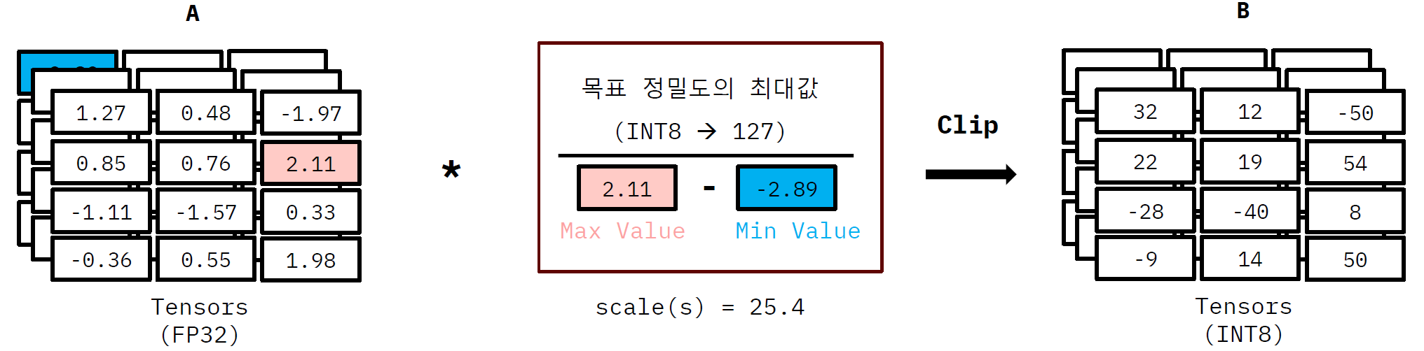
1. FP32 Tensor 행렬에서 Min, Max 값을 구하고 Min~Max 범위를 보정 범위라 한다.
2. Scale(s) 값 계산 (s = Max value of Int8 / (Max(A) - Min(A))
3. FP32 tensor 행렬의 각 tensor에 scale을 곱한 후 이를 반올림하여 INT8 값을 구한다.
Calibration
- 양자화 단계에서 보정 범위(Calibration Range)의 값이 어떻게 계산 되는지에 따라 이후 INT8 모델의 정확도에 영향을 미치게 됨.
- 보정 범위의 경우 아래 두가지 요소에 의해 크게 달라질 수 있으며, 모델에 맞는 데이터셋 구성과 계산 방법을 선택하는 것이 좋음.
- 1. Calibration Dataset
- 값의 분포가 다양한 Dataset을 구성하는 것이 이상적이나, Validation Dataset 일부를 사용하여 보정 범위를 계산
- 데이터 개수의 경우 늘려가면서 Quantization 이후 정확도 테스트를 진행하는 것을 추천.
- 2. Calibration Method
- 모델마다 적합한 Calibration Method가 다르기 때문에 최대한 많은 Calibration Method을 테스트 해보고 가장 정확도 저하가 낮은 Calibration Method을 탐색하는 과정이 필요
- 산출 방식
- Calibration Range 산출 방식
- 비히스토그램 기반 : 값 자체만 고려하는 방식
- 히스토그램 기반 : 값의 분포를 바탕으로 고려하는 방식
- Calibration Range 표현 방식
- 대칭형(SYM) : 범위를 대칭적으로 표현 (ex. [-a,a])
- 비대칭형(ASYM) : 범위를 비대칭적으로 표현 (ex.[-b, a])
- 성능
- Percentile_ASYM : 일반적으로 성능이 좋음
- MIN_MAX_ASYM : 가장 빠르게 Calibration Range 계산
- Calibration Range 산출 방식
- 1. Calibration Dataset
Optimize Quantized ONNX Graph


왼쪽 그림은 input data가 float 32일 때이며, 오른쪽 그림은 input / output data가 이미지거나 정수의 형태를 띌 때를 나타낸 그림입니다.
- 왼쪽 그림
- Quantize operator - float32 -> int8
- Dequantize operator - int8 -> float32
- 오른쪽 그림
- Quantize operator - uint8 -> int8
- 이 과정에서 Model Editor가 input data-> uint8로 바꿈
- CPU에서 동작을 더 빠르게 하기 위함
- 이 과정에서 Model Editor가 input data-> uint8로 바꿈
- Dequantize operator - int8 -> float32
- Quantize operator - uint8 -> int8
#furiosa_quantizer.py
import cv2
import os
import onnx

from tqdm import tqdm
from utils.preprocess import YOLOPreProcessor
from furiosa.optimizer import optimize_model
from furiosa.quantizer import (
    CalibrationMethod, Calibrator,quantize,
)

# Load ONNX Model
model = onnx.load("yolov8n.onnx")

# ONNX Graph Optimization
model = optimize_model(
    model = model,
    opset_version=13,
    input_shapes={"images": [1, 3, 640, 640]}
)

# FuriosaAI SDK Calibrator: onnx model, calibration method
calibrator = Calibrator(model, CalibrationMethod.MIN_MAX_ASYM)

data_dir = "../val2017"  #Import 10 images from this directory
calibration_dataset = os.listdir(data_dir)[:10]

# Preprocessing
preprocessor = YOLOPreProcessor()

for data_name in tqdm(calibration_dataset):
    data_path = os.path.join(data_dir, data_name)
    input_img = cv2.imread(data_path)
    input_, contexts = preprocessor(input_img, new_shape=(640, 640), tensor_type="float32")
    calibrator.collect_data([[input_]])

# Calculate Calibration Ranges
calibration_range = calibrator.compute_range()

# Quantization
quantized_model = quantize(model, calibration_range)

with open("yolov8n_i8.onnx", "wb") as f:
    f.write(bytes(quantized_model))
#furiosa_model_editor.py
import cv2
import os
import onnx
from tqdm import tqdm
from utils.preprocess import YOLOPreProcessor
from furiosa.optimizer import optimize_model
from furiosa.quantizer import (
CalibrationMethod, Calibrator, quantize,
ModelEditor, TensorType, get_pure_input_names,
)
# Load ONNX Model
model = onnx.load("yolov8n.onnx")
# ONNX Graph Optimization
model = optimize_model(
model = model, opset_version=13, input_shapes={"images": [1, 3, 640, 640]}
)
# FuriosaAI SDK Calibrator: onnx model, calibration method
calibrator = Calibrator(model, CalibrationMethod.MIN_MAX_ASYM)
data_dir = "../val2017"
calibration_dataset = os.listdir(data_dir)[:10]
# Preprocessing
preprocessor = YOLOPreProcessor()
for data_name in tqdm(calibration_dataset):
data_path = os.path.join(data_dir, data_name)
input_img = cv2.imread(data_path)
input_, contexts = preprocessor(input_img, new_shape=(640, 640), tensor_type="float32")
calibrator.collect_data([[input_]])
# Calculate Calibration Ranges
calibration_range = calibrator.compute_range()
# 추가된 부분
## Optimize Quantize Operator uinsg Model Editor
editor = ModelEditor(model)
input_names = get_pure_input_names(model)
for input_name in input_names:
editor.convert_input_type(input_name, TensorType.UINT8)
# Qauntization
quantized_model = quantize(model, calibration_range)
with open("yolov8n_opt_i8.onnx", "wb") as f:
f.write(bytes(quantized_model))

Quantize와 dequantize 과정에서 NPU와 CPU 간의 상호작용 방식에 대해 설명드리겠습니다.
- Quantize 과정:
- CPU에서 입력 데이터(float32)를 int8로 변환합니다.
- 이 변환된 int8 데이터는 NPU에서 효율적으로 처리될 수 있도록 준비됩니다.
- NPU에서 처리:
- 변환된 int8 데이터가 NPU에 입력되어, NPU는 이 데이터를 사용하여 고속 연산을 수행합니다.
- Dequantize 과정:
- NPU에서 계산된 int8 출력 데이터를 CPU로 반환한 후, CPU에서 이 데이터를 다시 float32로 변환합니다.
따라서, 전체 동작 과정은 CPU → NPU → CPU의 흐름으로 진행됩니다.
이 구조는 CPU와 NPU 간의 협력으로, 데이터 변환 및 연산을 최적화하여 성능을 향상시키는 방식입니다.
3. Runtime


Compiler : 양자화가 완료된 ONNX 파일을 입력으로 받아, FuriousAI NPU가 실행할 수 있는 형태의 프로그램으로 변환하는 도구
- DNN Model: 딥러닝 모델이 처음 입력으로 제공됩니다.
- Graph Optimization: 모델의 그래프 구조를 최적화하여 더 효율적으로 변경합니다.
- Parallelization: 병렬 처리를 위해 최적화된 그래프를 분석하고 변환합니다.
- Scheduling: 병렬 처리 계획을 수립하여 작업을 효율적으로 스케줄링합니다.
- Low-level Optimization: 하드웨어 수준의 최적화를 통해 성능을 향상시킵니다.
- Code Generation: 최적화된 모델을 실제 실행 가능한 코드로 생성합니다.
Furiosa Runtime은 NPU 실행, CPU 연산, 그리고 I/O 작업으로 구성된 종단 간 추론이 각각 독립적으로 실행할 수 있도록 합니다. 즉, 병렬처리가 가능하며 하드웨어 리소스를 최적화합니다.
- Runners/Queues
- Runners
- 동기(Sync) 또는 비동기(Async) 실행이 가능
- 작업을 실행하는 역할을 하는 run method 포함
- 한 번에 여러 개의 run 호출이 동시에 실행
- 동기 방식에서는 스레드를 사용
- 비동기 방식에서는 task 사용
- Queues
- 두 개의 클래스로 나뉨
- 데이터 보내기 위한 클래스 - send method (데이터를 큐에 보낼 때 사용)
- 데이터 받기 위한 클래스 - receive(recv) method (큐에서 데이터를 받을 때 사용)
- 각 send method 호출은 어떤 데이터가 어떤 문맥에서 보낸 것인지 구분할 수 있도록 도와주는 문맥 값(context value)과 함께 실행
- 두 개의 클래스로 나뉨
- Runners

왼쪽 그림은 sync, 오른쪽 그림은 async에 대한 설명입니다.
- Sync
- NPU가 일할 때 CPU는 쉬고 CPU가 일할 때 NPU가 동작을 안하기 때문에 비효율적입니다.
- Async
- 여러 개의 추론이 동시에 수행될 수 있습니다
- Sync의 경우보다 효율적입니다
이제 직접 시뮬레이션을 돌리며 알아보도록 하겠습니다.
Runners_sync
#furiosa_runners_sync.py
import os, subprocess, asyncio
import cv2
import time
import threading #for sync

from utils.preprocess import YOLOPreProcessor	#전처리
from utils.postprocess import ObjDetPostprocess #후처리
from furiosa.runtime.sync import create_runner  #모델을 실행하는 런타임 실행기 생성 함수

#주어진 모델 사용하여 이미지 처리 함수
def furiosa_runtime_sync(model_path, input_img, input_, contexts, data_name):
    postprocessor = ObjDetPostprocess()
    with create_runner(model_path, device = "warboy(2)*1") as runner: #warboy(2) means Warboy that has 2 NPU cores
        for _ in range(1000):										  #repeat 1000 times
            preds = runner.run([input_]) # FuriosaAI Runtime
            output_img = postprocessor(preds, contexts, input_img)	  #posstprocess the result of model prediction
            cv2.imwrite(os.path.join("result", data_name), output_img)#후처리된 이미지를 write하기


model_path = "yolov8n_opt_i8.onnx"
data_dir = "../val2017"
data_name = os.listdir(data_dir)[0]

if os.path.exists("result"):
    subprocess.run(["rm", "-rf", "result"])
os.makedirs("result")
#전처리
preprocessor = YOLOPreProcessor()
input_img = cv2.imread(os.path.join(data_dir, data_name))
input_, contexts = preprocessor(input_img, new_shape=(640, 640), tensor_type="uint8")

#Start Inference
t1 = time.time()
furiosa_runtime_sync(model_path, input_img, input_, contexts, data_name)
t2 = time.time()
print(f"Inference Time for 1000 images: {t2-t1}s")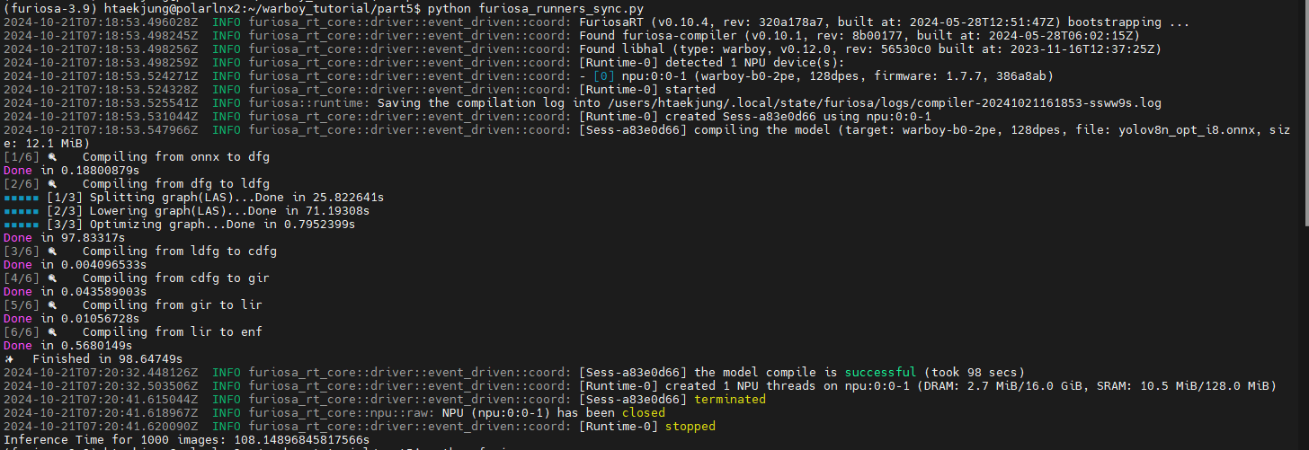
Sync의 경우 런타임 시간이 108.148초가 걸렸음을 알 수 있습니다.
Runners_async
#furiosa_runners_async.py
import os
import subprocess
import asyncio
import cv2
import time
from utils.preprocess import YOLOPreProcessor
from utils.postprocess import ObjDetPostprocess
from furiosa.runtime import create_runner

model_path = "yolov8n_opt_i8.onnx"
data_dir = "../val2017"
data_name = os.listdir(data_dir)[0]

if os.path.exists("result"):
    subprocess.run(["rm", "-rf", "result"])
os.makedirs("result")

preprocessor = YOLOPreProcessor()
input_img = cv2.imread(os.path.join(data_dir, data_name))
input_, contexts = preprocessor(input_img, new_shape=(640, 640), tensor_type="uint8")

async def inference(runner, input_img, input_, contexts, data_name, worker_id):
    postprocessor = ObjDetPostprocess()
    for i in range(1000):
        if i % 8 == worker_id:  # worker_id에 따라 작업 분배
            preds = await runner.run([input_])  # FuriosaAI Runtime
            output_img = postprocessor(preds, contexts, input_img)
            # Save each image with a unique name
            cv2.imwrite(os.path.join("result", f"{data_name}_worker{worker_id}_{i}.jpg"), output_img)

async def furiosa_runners_async(model_path, input_img, input_, contexts, data_name):
    async with create_runner(model_path, device="warboy(2)*1") as runner:
        await asyncio.gather(
            *(inference(runner, input_img, input_, contexts, data_name, idx) for idx in range(8))
        )

# Start timing
t1 = time.time()
asyncio.run(furiosa_runners_async(model_path, input_img, input_, contexts, data_name))
t2 = time.time()
print(f"Inference Time for 1000 images: {t2 - t1}s")
Async의 경우 런타임 시간이 5.956초가 걸렸음을 알 수 있습니다.
Queues_async
#furiosa_queues.py - async
import os, subprocess, asyncio
import cv2
import time
import threading

from utils.preprocess import YOLOPreProcessor
from utils.postprocess import ObjDetPostprocess
from furiosa.runtime import create_queue


async def submit_with(submitter, input_, contexts):
    for _ in range(1000):
        await submitter.submit(input_, context=(contexts))

async def recv_with(receiver, input_img, data_name):
    postprocessor = ObjDetPostprocess()
    for _ in range(1000):
        contexts, outputs = await receiver.recv()
        output_img = postprocessor(outputs, contexts, input_img)
        cv2.imwrite(os.path.join("result", data_name), output_img)

async def furiosa_runtime_queue(model_path, input_img, input_, contexts, data_name):

    async with create_queue(
        model=model_path, worker_num=8, device="warboy(2)*1"
    ) as (submitter, receiver):
        submit_task = asyncio.create_task(submit_with(submitter, input_, contexts))
        recv_task = asyncio.create_task(recv_with(receiver, input_img, data_name))
        await submit_task
        await recv_task


model_path = "yolov8n_opt_i8.onnx"
data_dir = "../val2017"
data_name = os.listdir(data_dir)[0]

if os.path.exists("result"):
    subprocess.run(["rm", "-rf", "result"])
os.makedirs("result")

preprocessor = YOLOPreProcessor()
input_img = cv2.imread(os.path.join(data_dir, data_name))
input_, contexts = preprocessor(input_img, new_shape=(640, 640), tensor_type="uint8")


t1 = time.time()
asyncio.run(furiosa_runtime_queue(model_path, input_img, input_, contexts, data_name))
t2 = time.time()
print(f"Inference Time for 1000 images: {t2-t1}s")
이 경우, 6.0668초가 걸렸음을 알 수 있습니다.
결론적으로 async인 경우가 sync인 경우보다 더 적은 시간이 걸렸음을 알 수 있습니다.
4. Debugger & Profiler


Warboy Application을 최적화하기 위해선 위와 같은 과정이 필요합니다.
Performance Testing
Evaluation Metrics
- 지연시간 (latency)
- 일반적으로 하나의 작업을 처리하는 데 걸리는 시간을 의미
- ML에서는 모델이 입력 데이터를 받아들이고 결과를 생성하는 데 걸리는 시간을 의미
- 빠른 반응 시간을 요구하는 서비스에서 중요하게 고려해야하는 평가 요소
- 처리량 (Throughput)
- 주어진 시간 동안 시스템이 처리하는 작업의 양을 의미
- ML에서는 주어진 시간 동안 모델이 얼마나 많은 추론 작업을 처리하는지를 나타내는 평가 요소
- 많은 작업량을 처리해야하는 서비스에서 중요하게 고려되어야 함
Vision application
- AI CCTV와 같은 Multi Channel Videos 처리하는 Vision Application의 경우, 지연시간보다 처리량이 조금 더 중요한 성능 요소임
Vision Application에서 처리량에 영향을 주는 부분
- Inference Latency: 추론에 걸리는 시간으로 하드웨어의 성능, 모델의 연산량 등에 영향을 받음
- Preprocessing: 추론에 사용하는 입력을 준비하는 작업 (e.g., Video -> Image Frame -> Input Tensor)
- Postprocessing: 추론 결과를 원하는 형태로 처리하는 작업 (e.g., Output Tensor -> Output Frame)
WARBOY Fusion | Single PE
- Fusion PE: Warboy 장치의 하드웨어 자원(SRAM 등)을 온전히 사용하기 때문에 모델을 실행할 때 낮은 latency를 얻을 수 있음
- 크기가 큰 모델의 경우 SRAM의 크기가 클수록 이점이 크기 때문에 Fusion PE를 사용하는 것이 좋음.
- Single PE : Warboy 장치의 하드웨어 자원을 나누어서 사용하기 때문에 Fusion PE보다 높은 latency를 지니게 되나, PE 2개를 병렬적으로 사용할 수도 있어 크기가 작은 모델의 경우 처리량(Throughput)이 더 높을 수 있음.
#furiosa-bench installation
sudo apt install furiosa-bench

# Usage of furiosa-bench
furiosa-bench model.onnx --workload T -n 1000 -b 8 -w 8 -t 8 -d npu0pe0,npu0pe1
위 코드를 통해 furiosa-bench를 설치한 다음 benchmark를 살펴보겠습니다.

- NPU : 관측 시간 중 NPU가 사용된 시간의 비율(100에 가까울수록 pre/postprocessing에서의 overhead가 적은 상태)
- overhead : 데이터를 처리하며 발생하는 추가적인 비용, 시간, 자원
- Comp : NPU가 차지하는 시간 중 실제 계산에 사용된 시간의 비율 (높을수록 Warboy에 친화적인 모델)
- I/O : NPU가 차지하는 시간 중 I/O에 사용된 비율(낮을수록 Warboy에 친화적인 모델)
위 benchmark를 통해 확인해봐야 할 것은 다음과 같습니다.
- Runtime을 측정했던 코드 furiosa_runners_sync.py, furiosa_runners_async.py, furiosa_queues.py를 실행시키며 얻은 벤치마크에서 어떠한 결과가 나타나는가?
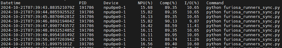
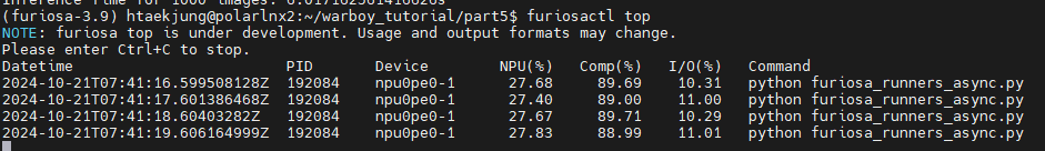
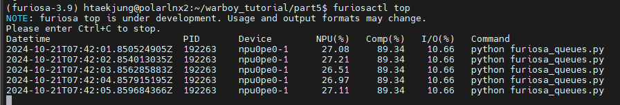
위 3개의 사진에서 볼 수 있듯이 Comp와 I/O 값은 모두 비슷하다는 것을 알 수 있지만 NPU 사용량이 async 코드를 실행시켰을 때 더 커서 NPU를 더 많이 사용한다는 것을 알 수있습니다.
본 포스트의 일부는 Furiosa 사의 Warboy tutorial 특강 강의자료에서 발췌하였습니다.
'프로젝트 & 경진대회' 카테고리의 다른 글
| Developing Vision Intelligence Applications on Furiosa WARBOY (0) | 2025.01.12 |
|---|---|
| Direct FIR Filter Digital Design in 2 versions with PPA results (0) | 2024.12.08 |
| Simplified FIR Filter Design (0) | 2024.11.30 |
| RISC-V Single-Cycle Processor Design (0) | 2024.10.12 |
| 차세대반도체 경진대회 회고록 (3) | 2024.09.08 |